Detecting Regime Changes Using Hidden Markov Models: The Case of Apple's Volatility

Introduction to Hidden Markov Models

Hidden Markov Models (HMMs) are statistical models that represent systems which transition between different states over time. At any given time, the system is assumed to be in one of these states, even though the exact state might be hidden or not directly observable. Instead, we can only observe some output that gives us clues about the underlying state. These models are particularly useful when you need to infer the underlying states of a system based on observable outputs, and the states are believed to follow a Markov process.

Hidden Markov Models (HMMs) offer a dynamic approach to detecting regime changes, as they inherently account for the temporal nature of sequential data, capturing shifts more effectively than static models (such as moving averages). Their ability to model unobserved states based on observable outcomes makes them superior, providing a nuanced understanding of underlying patterns without over-fitting.

Does Apple Normally Exhibit Higher Volatility When Reporting Earnings?

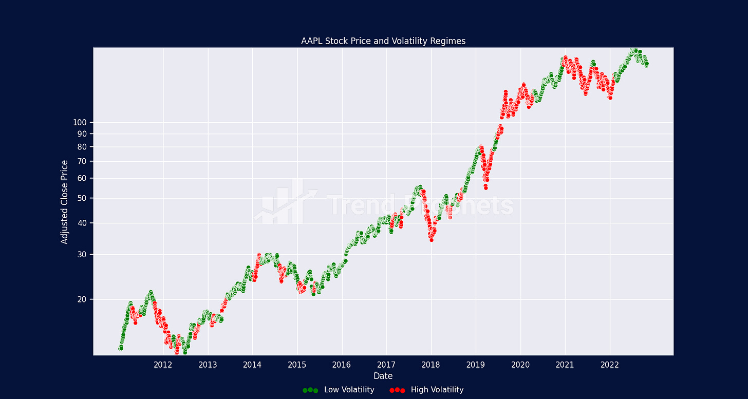
Using Apple's rolling 30-day volatility gives us a clear picture of market sentiment before its earnings announcements. By looking at this measure, we can see how the market feels about Apple's upcoming financial results. Since 2010, 60% of the time, Apple was in a low-volatility regime leading up to earnings. This raises an intriguing question: Is the market underestimating the chance of a surprise in Apple's earnings coming out on Thursday?

Figure 1: AAPL price since 2010. Green indicates a low volatility regime as identified using a Hidden Markov Model.

Low Volatility Persists in Most Major Indices

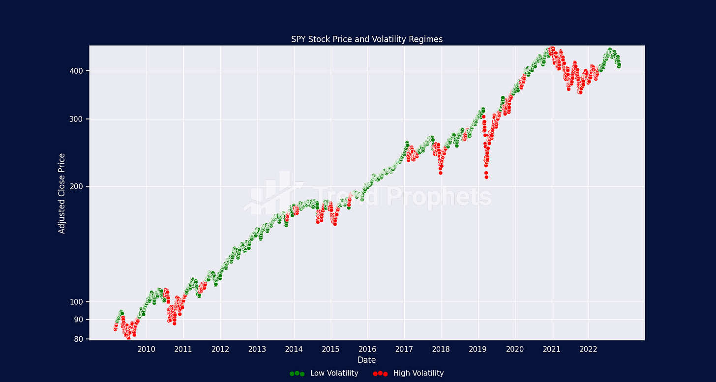
Of course, much of the current volatility seen in the mega-caps would mirror what we see in the broad based indices, especially given their high weights. Despite the 3-months of straight losses in SPY, we remain in a low volatility environment.

Figure 2: SPY price since 2010 with a Hidden Markov Model overlay identifying low and high volatility regimes.

Conclusion

Hidden Markov Models are potent tools for deciphering the hidden dynamics of time-series data, especially when many details remain unseen. They excel as predictive AI models and stand out as a crucial instrument for data scientists.

All data was retrieved from Yahoo! Finance using OpenBB.

Cordell Tanny, CFA, FRM, FDP is a co-founder and Chief Executive Officer of Trend Prophets, a quantitative and AI investment consulting service.

Disclaimer: Past results are no guarantee of future results and this is intended for informational purposes only.

trendprophets.com

https://www.linkedin.com/company/trend-prophets

Python code

import numpy as np
import pandas as pd
import matplotlib.pyplot as plt
from hmmlearn.hmm import GaussianHMM
from matplotlib.ticker import LogLocator
import seaborn as sns

sns.set()

"""
assuming you have downloaded the pricing data from your favourite data provider like OpenBB.
"""
# Calculate volatility (rolling standard deviation of returns, annualized)
df_aapl['volatility'] = df_aapl['adjusted_close'].pct_change().rolling(window=30).std() * np.sqrt(252)

df_aapl.dropna(inplace=True)

# Train HMM on volatility
model = GaussianHMM(n_components=2, covariance_type='full', n_iter=1000).fit(df_aapl['volatility'].dropna().values                                                                         .reshape(-1, 1))

# Predict the volatility regime
df_aapl['regime'] = model.predict(df_aapl['volatility'].dropna().values.reshape(-1, 1))

# Sorting the regimes by their means to ensure that regime 0 is low volatility and regime 1 is high volatility
if model.means_[0][0] > model.means_[1][0]:
    df_aapl['regime'] = df_aapl['regime'].map({0: 1, 1: 0})

# Plotting
fig, ax = plt.subplots(figsize=(15, 8))
sns.scatterplot(data=df_aapl, x=df_aapl.index, y='adjusted_close', hue='regime', palette=['green', 'red'], ax=ax)

ax.set_yscale('log')
# This will generate more ticks for the y-axis based on the range of your data
y_min, y_max = df_aapl['adjusted_close'].min(), df_aapl['adjusted_close'].max()
ax.yaxis.set_major_locator(LogLocator(base=10, subs='all', numticks=15))
ax.set_ylim(y_min, y_max)
ax.yaxis.set_major_formatter(plt.ScalarFormatter())  # This will remove scientific notation
ax.yaxis.tick_left()
ax.set_xticks(pd.date_range(start=df_aapl.index.min(), end=df_aapl.index.max(), freq='Y'))  # One tick per year
ax.set_xticklabels([date.strftime('%Y') for date in pd.date_range(start=df_aapl.index.min(), end=df_aapl.index.max(),
                                                                  freq='Y')])
ax.set_title('AAPL Stock Price and Volatility Regimes', loc='center')
ax.set_ylabel('Adjusted Close Price')
ax.set_xlabel('Date')
# Set legend properties for ax
handles, _ = ax.get_legend_handles_labels()
labels = ['Low Volatility', 'High Volatility']
legend = ax.legend(handles=handles, labels=labels, loc='upper center', bbox_to_anchor=(0.5, -0.08),
                   frameon=False, ncol=2)

plt.show()